dask-image: distributed image processing for large data

Presenter: Genevieve Buckley

Who needs dask-image?

If you're using numpy and/or scipy.ndimage and are running out of RAM, dask-image is for you.

Two main use cases

1. Batch processing
2. Large field of view

Motivating examples

• Sentinel satellite data
• Individual neurons within the brain

Getting started

https://github.com/dask/dask-image/

conda

conda install -c conda-forge dask-image

pip

pip install dask-image

What's included?

• imread
• ndfilters
• ndfourier
• ndmorph
• ndmeasure

Function coverage

GPU support

Latest release includes GPU support for the modules:

• ndfilters
• imread

Still to do: ndfourier, ndmeasure, ndmorph*

*Done, pending cupy PR #3907

GPU benchmarking

Architecture	Time
Single CPU Core	2hr 39min
Forty CPU Cores	11min 30s
One GPU	1min 37s
Eight GPUs	19s

https://blog.dask.org/2019/01/03/dask-array-gpus-first-steps

Let's build a pipeline!

1. Reading in data
2. Filtering images
3. Segmenting objects
4. Morphological operations
5. Measuring objects

%gui qt

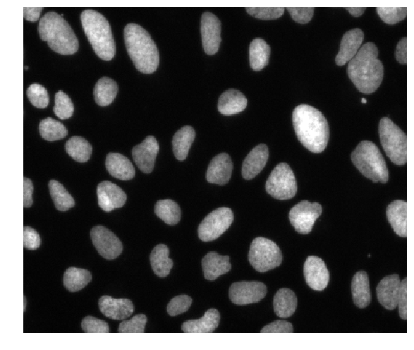
We used image set BBBC039v1 Caicedo et al. 2018, available from the Broad Bioimage Benchmark Collection Ljosa et al., Nature Methods, 2012.

https://bbbc.broadinstitute.org/BBBC039

1. Reading in data

from dask_image.imread import imread

images = imread('data/BBBC039/images/*.tif')
# images_on_gpu = imread('data/BBBC039/images/*.tif', arraytype="cupy")

images

Array Chunk Bytes 144.77 MB 723.84 kB Shape (200, 520, 696) (1, 520, 696) Count 600 Tasks 200 Chunks Type uint16 numpy.ndarray

2. Filtering images

Denoising images with a small blur can improve segmentation later on.

from dask_image import ndfilters

smoothed = ndfilters.gaussian_filter(images, sigma=[0, 1, 1])

3. Segmenting objects

Pixels below the threshold value are background.

absolute_threshold = smoothed > 160

# Let's have a look at the images
import napari
from napari.utils import nbscreenshot

viewer = napari.Viewer() 
viewer.add_image(absolute_threshold)
viewer.add_image(images, contrast_limits=[0, 2000])
nbscreenshot(viewer)

viewer.layers[-1].visible = False
napari.utils.nbscreenshot(viewer)

3. Segmenting objects (continued)

A better segmentation using local thresholding.

thresh = ndfilters.threshold_local(smoothed, images.chunksize)
threshold_images = smoothed > thresh

# Let's take a look at the images
viewer.add_image(threshold_images)
nbscreenshot(viewer)

4. Morphological operations

These are operations on the shape of a binary image.

https://docs.opencv.org/3.0-beta/doc/py_tutorials/py_imgproc/py_morphological_ops/py_morphological_ops.html

Erosion

Dilation

A morphological opening operation is an erosion, followed by a dilation.

from dask_image import ndmorph
import numpy as np

structuring_element = np.array([
    [[0, 0, 0], [0, 0, 0], [0, 0, 0]],
    [[0, 1, 0], [1, 1, 1], [0, 1, 0]],
    [[0, 0, 0], [0, 0, 0], [0, 0, 0]]])
binary_images = ndmorph.binary_opening(threshold_images, structure=structuring_element) 

5. Measuring objects

Each image has many individual nuclei, so for the sake of time we'll measure a small subset of the data.

from dask_image import ndmeasure

# Create labelled mask
label_images, num_features = ndmeasure.label(binary_images[:3], structuring_element)
index = np.arange(num_features - 1) + 1  # [1, 2, 3, ...num_features]
print("Number of nuclei:", num_features.compute())

Number of nuclei: 271

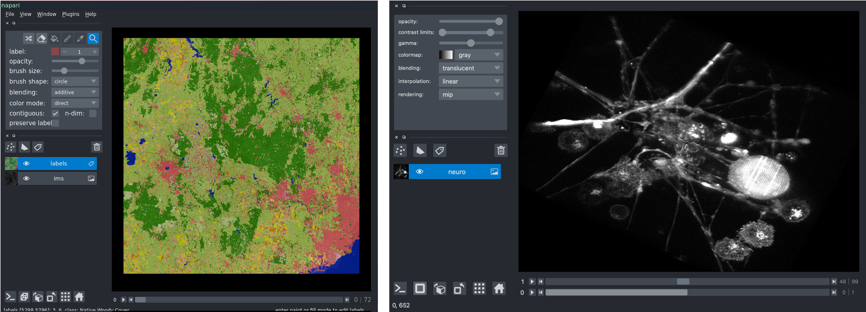
# Let's look at the labels
viewer.add_labels(label_images)
viewer.dims.set_point(0, 0)
nbscreenshot(viewer)